Creation of connector s-parameter model in the Clarity 3D simulation environment
The problem of the influence of connectors on signal integrity is extremely important, especially because of increasing data transmission speed in modern high-speed devices. However, it can be difficult to find s-parameter models that can be used to simulate the high-speed interface in time domain. At the same time, mechanical 3D models of connectors are usually available.
Creation of s-models can be carried out in two ways: the first is the extraction of models using a vector analyzer and a set of equipment with installed connectors, the second is the extraction of s-parameters by specialized calculation software (CAE). In this article we consider the second method.
The analysis process can be divided into several stages:
- Import of mechanical model;
- Preparation of design model;
- Determination of material properties;
- Assignment of signal and ground/power nets;
- Application of boundary conditions;
- Adjustment of calculation grid;
- Direct calculation;
- Processing of results.
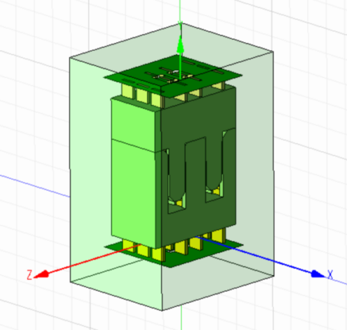
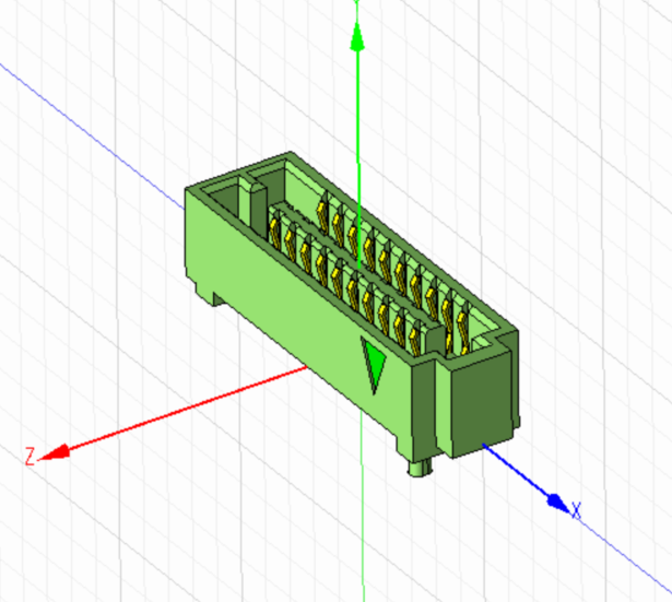
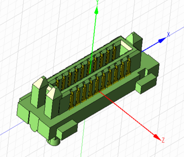
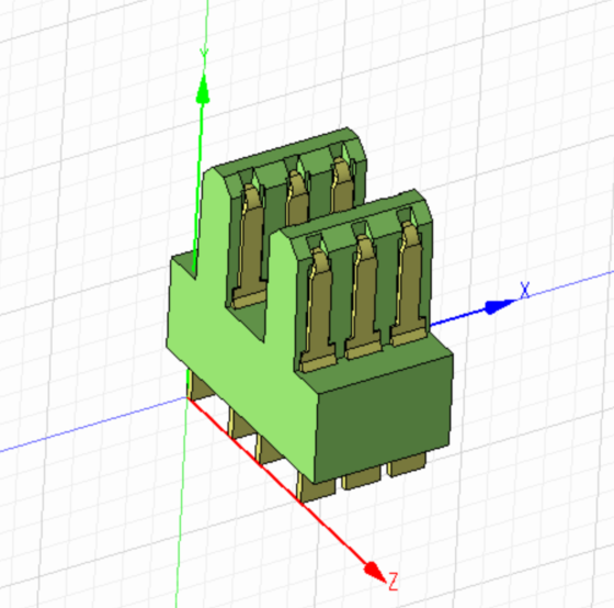
Figures 1a and 1b show the mechanical model imported into Clarity 3D from the STEP format and the prepared design model.
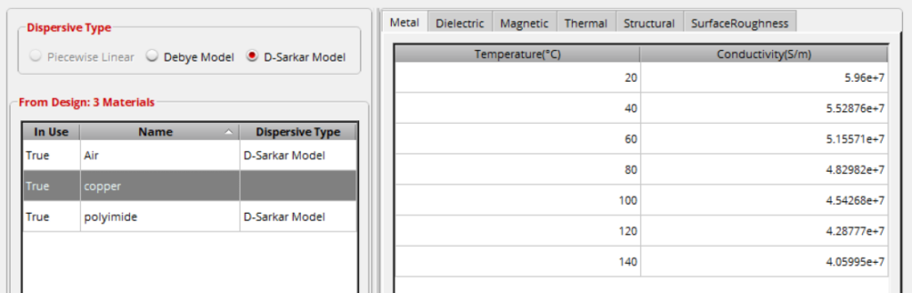
Modern CAEs have a fairly extensive libraries of materials. For this calculation, the following materials were selected: Air for the environment, Copper for contacts, Polyimide as the body material. Figure 2 shows library of project materials.
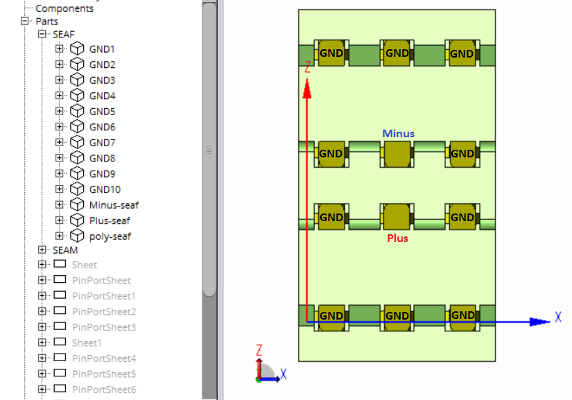
Further, the signal and ground circuits are assigned. Figure 3 shows the location of the contacts belonging to the respective circuits.
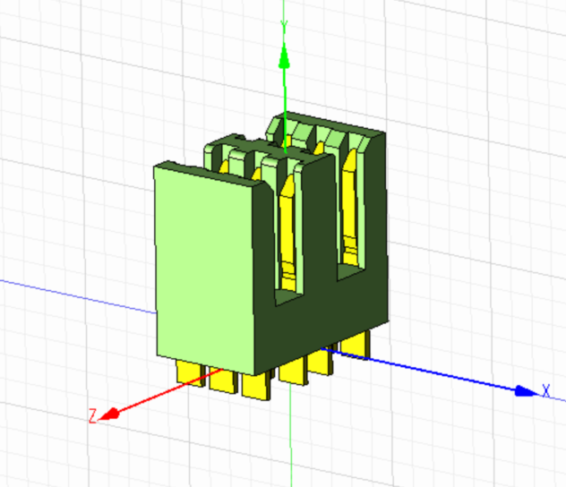
Due to the fact that the connector consists of two parts, the first four steps are repeated for the other part. Figures 4a and 4b show the imported mechanical model from the STEP format and the prepared design model.
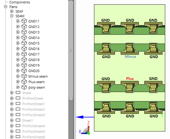
Further, the signal and ground nets are assigned. Figure 5 shows the location of the pins belonging to the respective nets.
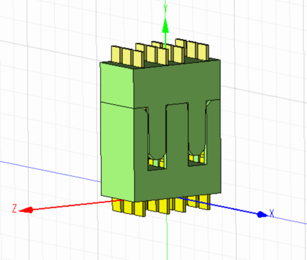
Both parts of the connector are combined into a single calculation model. Figure 6 shows the assembled calculation model.
The application of boundary conditions is shown in Figure 7.

The calculation grid is adjusted in such a way that the smallest element has at least 5 finite elements of design grid elements. Analyze is fulfilled in the frequency range up to 20 GHz at 10 MHz increments.
The following are the results of calculations.
Figures 8 and 9 show the transmission and reflection coefficients for the action in the differential mechanism.
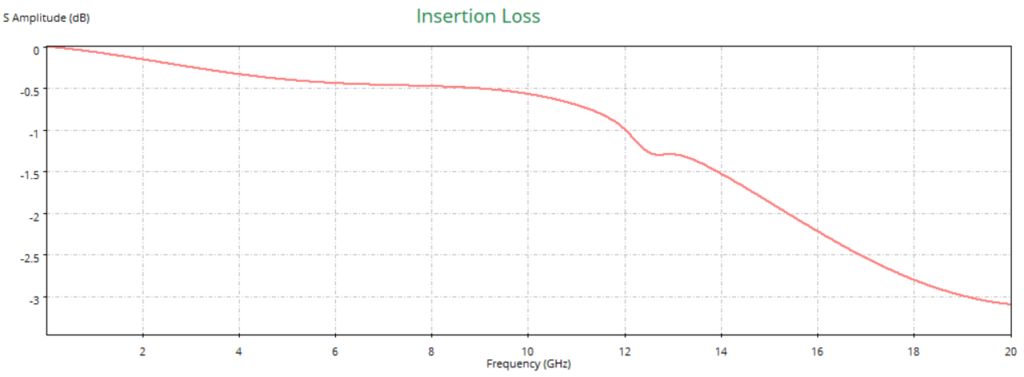
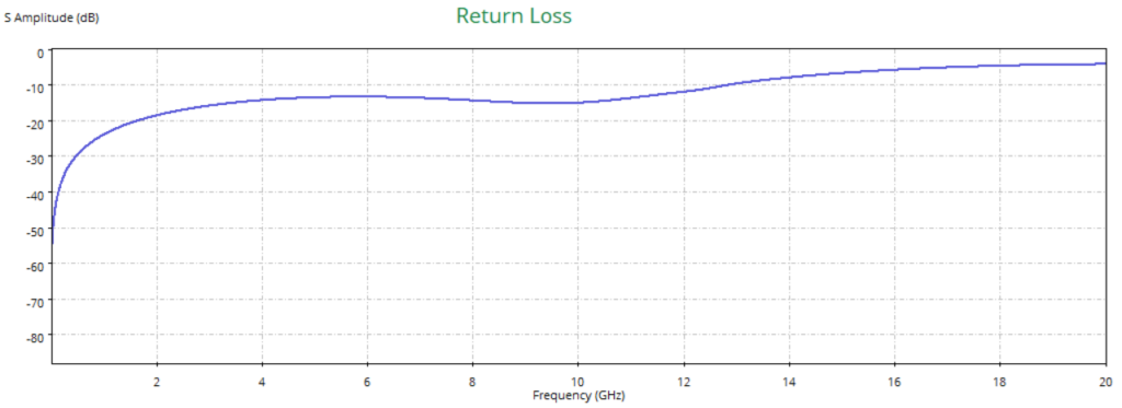
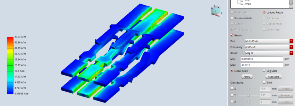
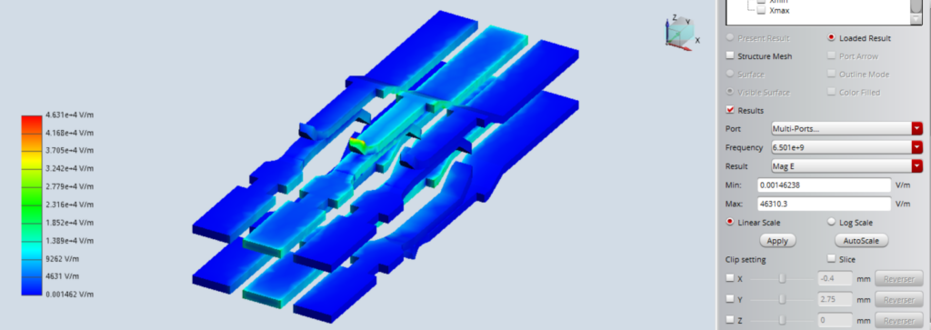
Figure 10 shows the magnetic field across conductive contacts. Figure 11 shows the electric field across conductive contacts.